Early Childhood Longitudinal Study

Relationships among demographic, social, and experiential variables and early achievement

What kinds of early childhood environments are associated with improved educational outcomes? The Early Childhood Longitudinal Study (Kindergarten class) looks at a variety of variables—cultural, socioeconomic, and educational—as they relate to early proficiency in reading and mathematics.

Our first step is to look at which variables are related to educational outcomes. Here, we will focus on children’s kindergarten math scores as our outcome of interest.

ESTIMATE COLUMNS FROM ecls ORDER BY DEPENDENCE PROBABILITY WITH C1R4MTSC LIMIT 15;

column	dependence probability with c1r4mtsc
c4r4rtsc	1.00
c1r4mtsc	1.00
c1r4rtsc	1.00
c4r4mtsc	0.98
wkmomed	0.77
wkdaded	0.77
wkpov_r	0.77
p2homecm	0.77
p1expect	0.75
race	0.75
p2safepl	0.73
p1prmlng	0.73
p2depres	0.69
p1chlboo	0.67
p1chlaud	0.67

After other math and reading scores, there are a collection of variables whose relationship to outcomes is rather intuitive. These include the mother and father’s education levels and expectations for tje child, wkmomed, wkmomed, p1expect, poverty level, wkpov_r, parents’ race and language, race and p1prmlng, whether a parent is depressed p2depres, and whether there is a computer in the home, p2homecm. However, for a small group of findings, it is less clear how they are related to math achievement. These include the number of books in the house, p1chlboo, and the number of CDs and tapes in the house, p1chlaud.

To investigate this further, we can explore how different values of each variable affect math scores. We will simulate predicted math scores given very small numbers of CDs and books (zero in each case), and given relatively large numbers of CDs and books (100 and 200, respectively). We have superimposed each pair of figures to compare the results, where the light blue represents zero and the gray represents large numbers of tapes and CDS or books.

PLOT SIMULATE C1R4MTSC FROM ecls GIVEN p1chlaud=0.00 TIMES 500 Save to simulate_C1R4MTSC_p1chlaud=0.png
PLOT SIMULATE C1R4MTSC FROM ecls GIVEN p1chlaud=100.00 TIMES 500 Save to simulate_C1R4MTSC_p1chlaud=100.png

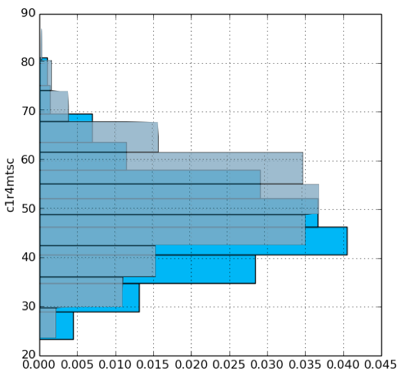
PLOT SIMULATE C1R4MTSC FROM ecls GIVEN p1chlboo=0.00 TIMES 500 Save to simulate_C1R4MTSC_p1chlboo=0.png
PLOT SIMULATE C1R4MTSC FROM ecls GIVEN p1chlboo=200.00 TIMES 500 Save to simulate_C1R4MTSC_p1chlboo=200.png

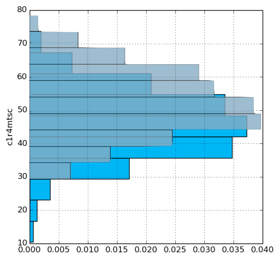
Larger numbers of tapes and CDs and larger numbers of books are both associated with higher scores. Indeed, our finding regarding books agrees with previous research showing that children that grow up around large numbers of books is related to educational performance (Evans et al., 2010).

References

[1] Evans, M. D. R., Kelley, J., Sikora, J. & Treiman, D. J. (2010). Family scholarly culture and educational success: Books and schooling in 27 nations. Research in Social Stratification and Mobility, 28(2), 171-197.

Dartmouth Atlas of Health

Recording the cost structure, capacity and quality of care of US hospitals.

One of the main concerns in American health care is addressing unwarranted variations in quality: a disparity between the cost and outcomes of care. The cost-care disparity is well-documented mainly as a result of the Dartmouth Atlas of Health Care, a freely available dataset which

…uses Medicare data to provide information and analysis about national, regional, and local markets, as well as hospitals and their affiliated physicians

These findings were the result of custom analysis by health economics and statistics researchers. Here we will see how easy it is to answer the same underlying questions using BayesDB.

Unwarranted variations in aggregate

First, we create a btable and load in pre-computed models,

CREATE BTABLE dha FROM dha.csv;
LOAD MODELS dha_models.pkl.gz INTO dha;

To get a sense of the probable dependencies between variables, we create a column dependence probability matrix in which each cell represents a pair of variables and the value represents the probability of their being statistically dependent under the inferred CrossCat model. Here, we have zoomed in on two variables, the first related to Medicare spending, and the second related to quality.

ESTIMATE PAIRWISE DEPENDENCE PROBABILITY FROM dha SAVE TO dha_z.png;

The resulting figure plots dependence probabilities of all pairs of variables as saturations in a large matrix. Dark areas represent variables with a high probability of dependence, light areas indicate a low probability of dependence. This contains quite a bit more information than we need, so we select out the rows that correspond to two variables that represent our question of interest: Medicare spending on ambulances and quality of care.

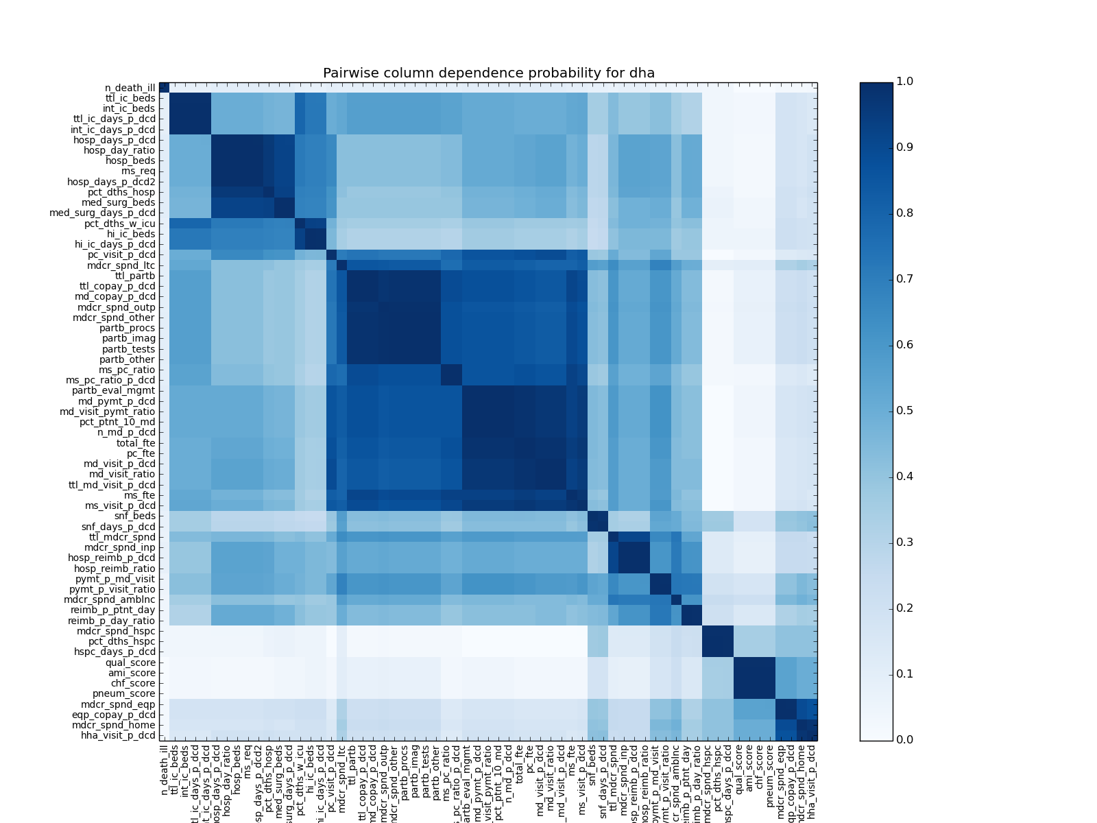
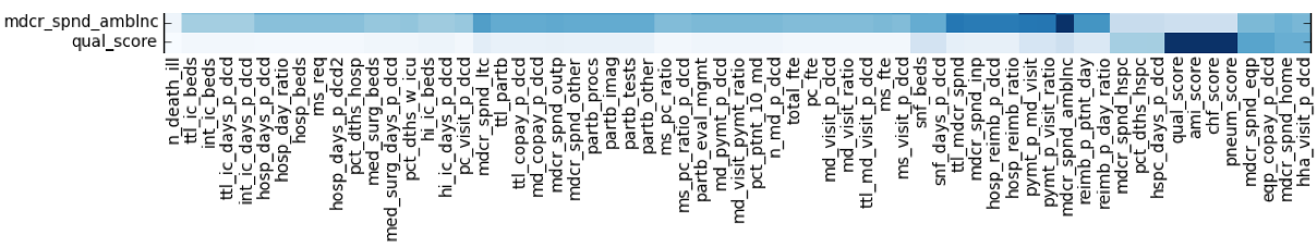
Notice that quality and cost show no dependence. We can list the variables that probably have a dependence on spending, again focusing on Medicare spending on ambulances.

ESTIMATE COLUMNS FROM dha ORDER BY DEPENDENCE PROBABILITY WITH mdcr_spnd_amblnc LIMIT 10

column	dependence probability with mdcr_spnd_amblnc
mdcr_spnd_amblnc	1.00
pymt_p_visit_ratio	0.73
ttl_mdcr_spnd	0.73
pymt_p_md_visit	0.73
mdcr_spnd_inp	0.71
hosp_reimb_ratio	0.71
hosp_reimb_p_dcd	0.71
reimb_p_day_ratio	0.61
reimb_p_ptnt_day	0.61
mdcr_spnd_ltc	0.57

Other spending variables as well as reimbursement related tend to be dependent, while quality variables do not appear on the list.

Similarly, we can list the variables that have the highest probability of dependence with quality,

ESTIMATE COLUMNS FROM dha ORDER BY DEPENDENCE PROBABILITY WITH qual_score LIMIT 10

column	dependence probability with qual_score
ami_score	1.00
qual_score	1.00
pneum_score	1.00
chf_score	1.00
mdcr_spnd_eqp	0.55
eqp_copay_p_dcd	0.55
mdcr_spnd_home	0.50
hha_visit_p_dcd	0.50
mdcr_spnd_hspc	0.34
pct_dths_hspc	0.34

The list includes other quality related scores, which have a very strong dependence. All of the remaining variables do not show strong evidence of dependence.

Unwarranted variations on a per-town basis

Which hospitals have surprising spending and quality levels — either unusually low or unusually high — given their other attributes?

SELECT name, PREDICTIVE PROBABILITY OF mdcr_spnd_amblnc FROM dha ORDER BY PREDICTIVE PROBABILITY OF mdcr_spnd_amblnc ASC LIMIT 10

name	predictive probability mdcr_spnd_amblnc
McAllen TX	2.68e-05
Beaumont TX	3.62e-05
Worcester MA	6.35e-05
Corpus Christi TX	1.27e-04
Panama City FL	1.99e-04
Temple TX	2.43e-04
Tupelo MS	2.47e-04
Takoma Park MD	2.60e-04
Tyler TX	3.36e-04
Houston TX	3.46e-04

SELECT name, PREDICTIVE PROBABILITY OF qual_score FROM dha ORDER BY PREDICTIVE PROBABILITY OF qual_score ASC LIMIT 10

name	predictive probability qual_score
Minot ND	0.05
Elyria OH	0.08
Muncie IN	0.08
Chicago IL	0.10
McAllen TX	0.10
El Paso TX	0.10
Monroe LA	0.10
Lake Charles LA	0.11
New Brunswick NJ	0.11
Abilene TX	0.11

McAllen TX appears on both lists as being suprising with respect to Medicare spending on ambulances and with respect to quality of care. To check this result, we might look at some more generic assessment of spending, such as the payment received per doctor’s visit.

SELECT name, PREDICTIVE PROBABILITY OF pymt_p_md_visit FROM dha ORDER BY PREDICTIVE PROBABILITY OF pymt_p_md_visit ASC LIMIT 10

name	predictive probability pymt_p_md_visit
Owensboro KY	0.02
McAllen TX	0.02
Everett WA	0.02
Manchester NH	0.03
Springdale AR	0.03
Portland OR	0.03
Dubuque IA	0.03
Santa Rosa CA	0.03
Olympia WA	0.03
New Orleans LA	0.03

Only one of these hospitals, McAllen TX, appears on all three of these lists. It has also been repeatedly written up in the popular press (The NewYorker, CBS News and NPR) as an illustration of the dissociation between spending and quality of care.

Further information

The BayesDB-ready .csv and pre-computed models used here can be found in the /examples directory in the BayesDB Github Repository.

For more information about the Dartmouth Atlas of Health Care, http://www.dartmouthatlas.org/.

General Social Survey

Responses to ~5500 demographic, behavioral and attitudinal questions by US residents.

The General Social Survey is conducted annually to assess the demographics and attitudes of U.S. residents. Questions span current housing situations, religion, voting, and positions on social issues. It aims to cover social attitudes and demographic variables such that their covariation can be studied. We are going to use BayesDB to explore this data, first to simply explore some relatively familiar variables for which we might have strong intuitions, second to assess BayesDB’s inferences against findings from other research, and finally to generate hypothetical survey responses.

What variables are associated with born-again experiences?

Religion is one topic for which we have strong intuitions, and it therefore is a useful case to assess the quality of BayesDB’s inferences. The GSS contains a number of questions related to religion. Here, we focus on people’s responses to the question of whether they have had a born-again experience. This is a feature of Christian religions, and especially Evangelical religions. We begin by ordering the variables based on the inferred dependence probability.

ESTIMATE COLUMNS FROM gss_pared ORDER BY DEPENDENCE PROBABILITY WITH reborn LIMIT 10

column	dependence probability with reborn
savesoul	1.00
reborn	1.00
evolved	1.00
god	0.98
bible	0.98
bigbang	0.98
prayer	0.94
postlife	0.94
homosex	0.92
grass	0.90

We can see that a number of variables are inferred to be probably dependent. These include whether one tries to convince others to accept Jesus Christ, believes that humans evolved from animals, believes in God, believes the bible is the word of God, believes in the Big Bang, prays, believes in the afterlife, believes homosexuality is wrong, and believes that marijuana should be legalized. These inferred dependencies span a variety of domains, from purely religious issues to morals, science, and public policy. With the possible exception of the legalization of marijuana, these inferences are quite consonant with intuition.

We can take a closer look at the relationship between born-again experiences and beliefs about the legalization of marijuana.

PLOT SELECT reborn, grass FROM gss_pared SAVE TO select_reborn_grass.png

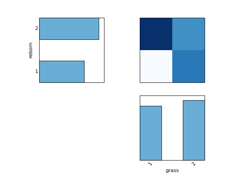
If one favors legalization, it is highly probable that one has not had a born-again experience. Interestingly, people who do not favor legalization may or may not have had a born-again experience. Taking a closer look at marijuana legalization,

ESTIMATE COLUMNS FROM gss_pared ORDER BY DEPENDENCE PROBABILITY WITH grass LIMIT 10

column	dependence probability with grass
grass	1.00
homosex	0.98
suicide1	0.96
letdie1	0.94
prayer	0.92
savesoul	0.90
reborn	0.90
evolved	0.90
god	0.88
bible	0.88

we see a largely complementary set of results. The first three variables are related to moral issues: homosexuality and whether suicide should be allowable under different circumstances. The remaining variables are religious, with the exception of the issue of evolution, which we know to be strongly related to religous beliefs.

Are homeowners more likely to vote?

Turning to a documented finding, economics research has shown that homeowners engage more in community activities than renters. They are also more likely to vote, more likely to know the names of the local political representatives, and more likely to engage in civic activities (DiPasquale, D., & Glaeser, E. L., 1999). For this reason, homeowners have been labeled better citizens (DiPasquale, D., & Glaeser, E. L., 1999; McCabe, 2013).

First we shall check whether the homeowners of 2012 are more likely to vote than renters. Since we are using the 2012 GSS we’ll investigate the relationship between vote08 and dwelown variables. vote08 is a categorical variable, where 1 indicates that the respondent voted in the 2008 presidential election, while 0 indicates that the did not. dwelown is also a categorical variable where 1 indicates that the respondent owns their home, and 2 indicates that the respondent rents their home.

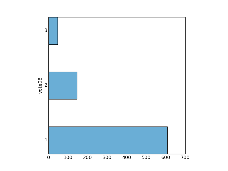
First, for homeowners (dwelown=1),

PLOT SELECT vote08 FROM gss_pared where dwelown=1 SAVE TO votedwel_1.png;

and second, for renters (dwelown=2)

PLOT SELECT vote08 FROM gss_pared where dwelown=2 SAVE TO votedwel_2.png;

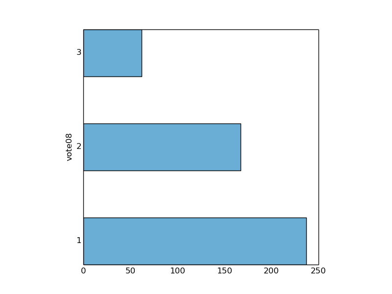
We see that 75% of homeowners voted while only 50% of renters voted.

Generating hypothetical survey responses

An interesting feature of BayesDB is the ability to simulate hypothetical data based on what it has learned from the observed data. Here we use this feature to assess the quality of BayesDBs predictions. We focus on a subset of the variables discussed above:

SIMULATE reborn, savesoul, bible, evolved FROM gss_pared TIMES 10

reborn	savesoul	bible	evolved
No	No	Inspired word	T
No	No	Ancient book	T
No	No	Ancient book	T
No	No	Inspired word	T
No	No	Ancient book	T
No	Yes	Ancient book	T
No	Yes	Actual word	F
Yes	No	Inspired word	T
Yes	Yes	Actual word	F
Yes	Yes	Actual word	F

We have sorted the simulated responses based on the first two columns. At the top are cases where the simulated respondant did not have a born-again experience and has not encouraged someone to accept Jesus. For this group, we see strong consensus responses on the other two questions: they believe the bible is not the actual word of God and that humans evolved from animals. In contrast, the simluated respondants who had had born-again experiences and had encouraged someone to accept Jesus responded that the bible is the actual word of God and that humans did not evolved.

We can further investigate the relationship by simulating the values of some variables, given the values of others. For example, we can simulate the same variables given that the individual believes humans evolved from animals, and again given that an individual believes that the bible is the actual word of God.

SIMULATE reborn, savesoul, bible, evolved FROM gss_pared GIVEN evolved=2 TIMES 10

reborn	savesoul	bible	evolved
No	Yes	Actual word	F
Yes	No	Ancient book	F
Yes	No	Inspired word	F
Yes	Yes	Actual word	F
No	Yes	Ancient book	F
No	Yes	Actual word	F
Yes	Yes	Inspired word	F
Yes	Yes	Actual word	F
Yes	Yes	Actual word	F
No	No	Actual word	F

SIMULATE reborn, savesoul, bible, evolved FROM gss_pared GIVEN bible=1 TIMES 10

reborn	savesoul	bible	evolved
Yes	Yes	Actual word	F
Yes	Yes	Actual word	F
No	No	Actual word	F
Yes	Yes	Actual word	F
No	No	Actual word	T
Yes	Yes	Actual word	F
Yes	Yes	Actual word	F
Yes	Yes	Actual word	F
Yes	No	Actual word	T
No	Yes	Actual word	T

In the first simulation, conditioning on the belief that humans did not evolve from animals elicits a change toward the belief that the bible is the actual word of God. Similary, conditioning on the belief that the bible is the actual word of God elicits a shift toward a belief that humans did not evolve from animals.

References

[1] DiPasquale, D., & Glaeser, E. L. (1999). Incentives and social capital: are homeowners better citizens? Journal of urban Economics, 45(2), 354-384.

[2] McCabe, B. J. (2013). Are Homeowners Better Citizens? Homeownership and Community Participation in the United States. Social forces, sos185.

Further information

The full GSS dataset can be downloaded from their website, here.